**DawgTide** DawgTide is a windsurfing-optimized dashboard of daily tides for the San Francisco Bay Area. It gives a high-level overview of the water level and current conditions at the windsurfing sites most affected by tides (e.g. Crissy Field, Haskins, and others). [DawgTide](http://winds.leverich.org/dawgtide/) is the successor to [Tidely](http://winds.leverich.org/tidely/). It is written entirely in Javascript and HTML/CSS (including harmonic tide prediction). https://github.com/leverich/dawgtide/ # Basic Usage Each "Tide Box" in DawgTide gives a snapshot overview of the tide situation from 2pm to 6pm, the prime sailing window during the summer. Clicking on any box goes to a detailed view for that location with a tide table and graph for daylight hours. For stations sensitive to water level (e.g. Haskins, Palo Alto, 3rd Avenue), we set a benchmark water level above which sailing is "Safe". Sailing when the water is below this level isn't necessarily "Unsafe", but you may have a really, really bad day (e.g. crawling 100 yards through mud at Palo Alto). Use your own judgement. 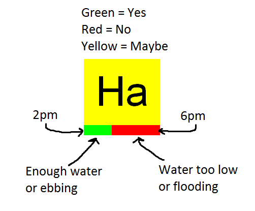For stations sensitive to current (e.g. Crissy Field, Treasure Island, 3rd Avenue, Sherman Island, Palo Alto), "Ebbing" is good (green), "Flooding" is bad (red). 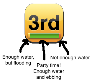For stations sensitive to both tide and current (3rd Ave and Palo Alto), green indicates enough water and ebbing, yellow indicates enough water and *flooding*, and red indicates water too low. # Stations Site | Reference | Coordinates --------------------------|--------------------------------|----------------------- Haskins (tide) | [Oyster Point Marina](https://co-ops.nos.noaa.gov/stationhome.html?id=9414392) | 37.664964, -122.376688 Golden Gate (current) | [Golden Gate Bridge (0.46 nm E)](http://tidesandcurrents.noaa.gov/noaacurrents/Predictions?id=SFB1203_18) | 37.8201, -122.4730 Treasure Island (current) | [Treasure Island (0.78 nm NW)](http://tidesandcurrents.noaa.gov/noaacurrents/Predictions?id=SFB1210_13) | 37.8373, -122.3872 3rd Avenue (tide) | [San Mateo Bridge](https://co-ops.nos.noaa.gov/stationhome.html?id=9414458) | 37.579991, -122.253344 3rd Avenue (current) | [San Mateo Bridge](http://tidesandcurrents.noaa.gov/noaacurrents/Predictions?id=SFB1305_7) | 37.5878, -122.2502 Palo Alto (tide) | [Coyote Creek, Alviso Slough](https://co-ops.nos.noaa.gov/stationhome.html?id=9414575) | 37.465000, -122.023323 Palo Alto (current) | [Dumbarton Bridge](http://tidesandcurrents.noaa.gov/noaacurrents/Predictions?id=SFB1301_12) | 37.5018, -122.1160 Delta (current) | [Sherman River Light 14](http://tidesandcurrents.noaa.gov/noaacurrents/Predictions?id=SFB1332_15) | 38.0772, -121.7639 To predict water levels "tide" stations, the harmonic constituents published by NOAA (e.g. [https://co-ops.nos.noaa.gov/harcon.html?id=9414392](https://co-ops.nos.noaa.gov/harcon.html?id=9414392)) are used as-is. To predict speeds for "current" stations, harmonic constituents are estimated from NOAA predictions using the method described below. ## Map https://goo.gl/Ikzq06 https://www.google.com/maps/d/viewer?mid=zuRpQMcYORZo.kEH83Bs1mltc # Fitting Harmonic Constituents from Data Given timestamped data from a tide station, we can fit the components of a [tidal harmonic model](https://en.wikipedia.org/wiki/Theory_of_tides#Harmonic_analysis) using plain linear regression (ordinary least squares). The harmonic model of tides for a station \(s\) at time \(t\) (relative to some reference year \(Y\)) for the [37 constituents](https://en.wikipedia.org/wiki/Theory_of_tides#Tidal_constituents) used by NOAA/NOS is: $$ y(s,t,Y) = Z_s + \sum_{i=1}^{37} a_{s,i} \cdot n_{Y,i} \cdot \textrm{cos}(t \cdot \omega_i + \Phi_{Y,i} - \phi_{s,i}) $$ where: * \(s\) is a tide station (e.g. "San Francisco, CA", 9414290). * \(t\) is a timestamp in seconds since Jan 1 \(Y\) 00:00 UTC. * \(Y\) is the year of the prediction. * \(Z_s\) is the mean tide value for station \(s\) (e.g. mean sea level relative to some "[datum](https://tidesandcurrents.noaa.gov/datum_options.html)", or average current). * \(a_{s,i}\) is the amplitude for coefficient \(i\), station \(s\). Typically reported in feet for tide height, knots for tidal current. * \(n_{Y,i}\) is the "node factor" for coefficient \(i\) for year \(Y\) (based on the [Moon's nodal period](https://en.wikipedia.org/wiki/Lunar_node) of ~18.61 years). Unitless. This is computed using [tide_fac.f](https://gist.github.com/leverich/e0834df944d457962a4e), which follows the methodology of [Schureman](http://docs.lib.noaa.gov/rescue/cgs_specpubs/QB275U35no981940.pdf). * \(\omega_i\) is the speed for coefficient \(i\) (radians per second). Often reported in degrees per hour. * \(\Phi_{Y,i}\) is the "equilibrium" phase "\(V_0 + U\)" for coefficient \(i\), year \(Y\) (radians). Often reported in degrees. This is computed using [tide_fac.f](https://gist.github.com/leverich/e0834df944d457962a4e), which follows the methodology of [Schureman](http://docs.lib.noaa.gov/rescue/cgs_specpubs/QB275U35no981940.pdf). * \(\phi_{s,i}\) is the phase for coefficient \(i\), station \(s\) (radians). Often reported in degrees. Note that this model is complicated by the presence of the "lookup tables" \(n\) and \(\Phi\). This is a peculiar artifact of [Schureman's](http://docs.lib.noaa.gov/rescue/cgs_specpubs/QB275U35no981940.pdf) methodology, for which he provided exhaustive tables of constants in various appendices. It's particularly annoying that all of the phases are effectively referenced from Jan 1 of a specific year, rather than a fixed point in the past (e.g. the UNIX epoch, Jan 1 1970 00:00 UTC). Be especially careful when algebraically manipulating this model to keep track of the reference time used for timestamps and phases. ## Estimating \(a\) and \(\phi\) To fit parameters to the harmonic model given above, we only need to solve for \(a_{s,i}\) and \(\phi_{s,i}\) for \(i=1 \ldots 37\) (the 37 constituents reported by NOAA/NOS), as \(n_{Y,i}\), \(\Phi_{Y,i}\), \(\omega_i\), and \(t\) are all known parameters. However, because of the unknown parameter within the \(\textrm{cos}\), this is not a linear system, so we can't directly solve for it with least squares. Instead, we solve for \(A_{s,i}\), \(B_{s,i}\) in a model of the form: $$ y(s,t,Y) = Z_s + \sum_{i=1}^{37} \left(A_{s,i} \cdot n_{Y,i} \cdot \textrm{sin}(t \cdot \omega_i + \Phi_{Y,i}) + B_{s,i} \cdot n_{Y,i} \cdot \textrm{cos}(t \cdot \omega_i + \Phi_{Y,i})\right) $$ Note that the terms other than \(A_{s,i}\) and \(B_{s,i}\) are known and constant, so this is trivially optimized with a least squares solver. Then, using the trigonometric identity: $$ A \cdot \textrm{sin}(\theta) + B \cdot \textrm{cos}(\theta) = \sqrt{A^2+B^2} \cdot \textrm{cos}\left(\theta + \textrm{atan2}(B_{s,i},A_{s,i}) - \frac{\pi}{2}\right)$$ we solve for \(a_{s,i}\) and \(\phi_{s,i}\) algebraically as: $$ a_{s,i} = \sqrt{A_{s,i}^2 + B_{s,i}^2} $$ $$ \phi_{s,i} = -\textrm{atan2}(B_{s,i},A_{s,i}) + \frac{\pi}{2} $$